Example Code
Download the complete reproduction package or the Python source. The saved run used Python 3.12.14.
This program studies the thermodynamic driving force, or affinity, needed when an autocatalytic network produces X at its greatest steady rate. It starts with reaction counts, constructs rate constants, checks the steady state and its responses, and verifies algebraic identities that prove the stated global maxima. The figures show actual saved calculations, so no installation is needed to inspect the results.
The main result in numbers
Holding X at a chosen concentration x and allowing Y to settle, consider X ⇌ Y with rate constants (3,2), and 2Y ⇌ 2X+Y with rate constants (7,6), the unique greatest production rate occurs at x=y=1. The forward rates are 3 and 7, the reverse rates are 2 and 6, and both net reaction currents equal 1. Thus Y is stationary and the net production of X is −1+2=1.
The dimensionless affinity measures forward driving through the log ratio of forward to reverse rates. At this maximum it is
below the conjectured minimum log(2) ≈ 0.6931471806. This comparison concerns a maximum of the production rate, not a minimum of affinity along that one network's entire steady-state curve.
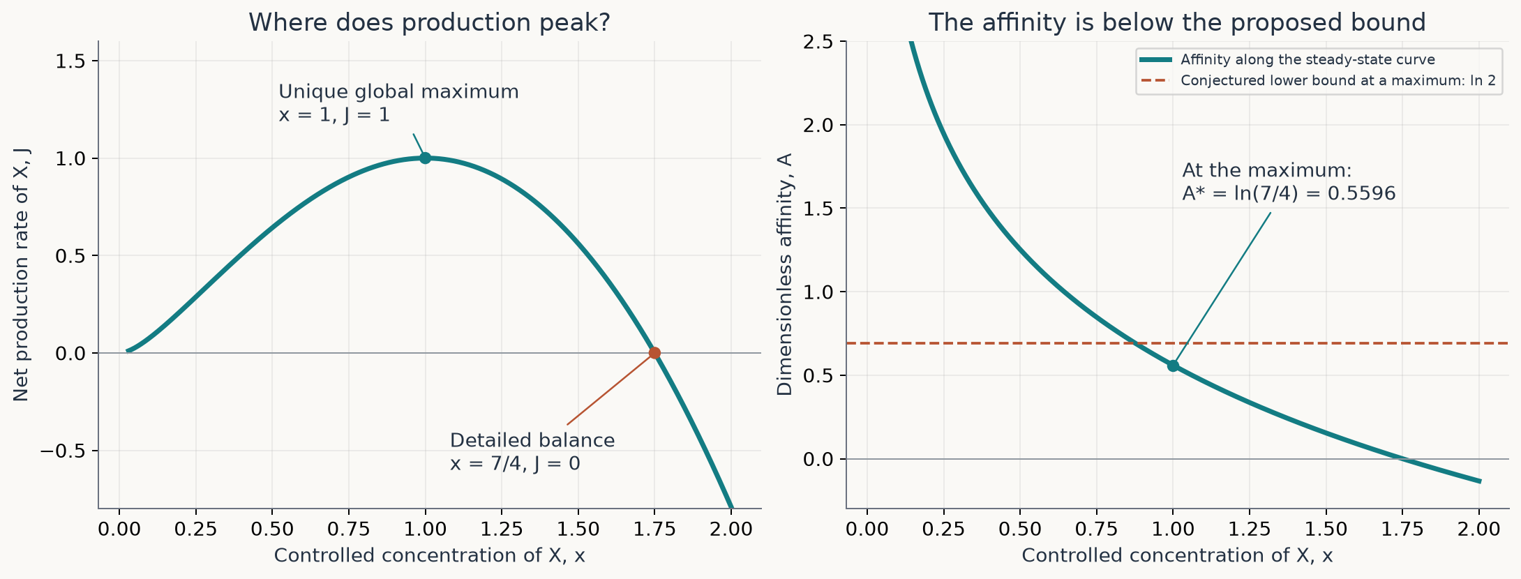
The left panel shows production. The right shows affinity at the same steady states. At x=7/4 the system reaches detailed balance, with zero net production and zero affinity. The plotted window is finite; the following identity proves the global conclusion for every positive steady state.
Set E=3x−2y−7y²+6x²y, s=2y, and J=3x−2y. The program checks exactly that
At a steady state E=0 and s>0. If J>1, the right side is positive, a contradiction. If J=1, it forces s=2, hence x=y=1. This is why an algebraic identity, together with its sign argument, establishes a global maximum rather than merely suggesting one from a graph.
The same molecule count permits very different affinities
The family X ⇌ Y, mY ⇌ 2X+(m−1)Y always has the same overall X count: one consumed and two produced. Choose an integer m≥2 and 1<r<2, and set
The unique global maximum is still at x=y=1 with J=1, but its affinity satisfies
Here r is the derivative of log y with respect to log x at the maximum. It measures the relative concentration response, not a reaction-rate constant.
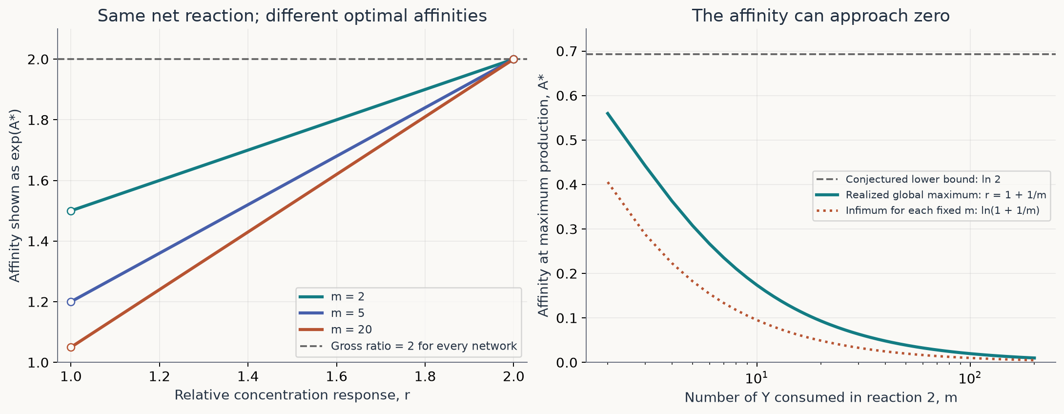
For each fixed m, the lowest limit of exp(A*) is 1+1/m, approached as r decreases toward 1. The endpoint is excluded. Along r=1+1/m the realized value is 1+2/m−1/m², which tends to 1; its logarithm therefore tends to zero. This limit changes m and the rate constants. At the displayed normalization J=1, some rates become large.
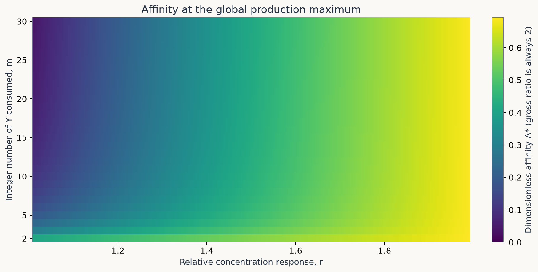
The map evaluates the exact formula on 29 integer values of m and 197 values of r. Color represents A*, not exp(A*). The map shows affinity, rather than classifying different kinds of dynamics. CSV files contain the plotted numbers.
How the code constructs an actual local maximum
The generic reconstruct function accepts the reactant counts, product counts and a requested forward-response vector f. It normalizes that vector so that log x increases at unit speed, calculates the reverse responses h and the ratios qᵢ=hᵢ/fᵢ, and sets
All monomials equal one at unit concentrations, so these rate constants are also the one-way rates at the constructed state. The code then checks positivity, stationarity, zero first derivatives, the rank of the current Jacobian, regularity of the controlled stationary equations, and the strictly negative second derivative of production.
For the main example the results are f=(1,3), h=(3/2,7/2), q=(3/2,7/6), and d²J/d(log x)²=−33/10. The routing weights give the same curvature as direct second differentiation of the stationary equations. An independent numerical solve at log x=±0.001 gives a finite-difference curvature of approximately −3.30000238; its error relative to −3.3 is about 2.38×10⁻⁶.
The general theorem requires the hypotheses listed in the demonstration plan and Theorem 5.15. Checking those hypotheses for one supplied profile does not prove that every profile in an arbitrary source's allowed set is accessible. Nor does the local construction establish global optimality without another argument.
Additional exact examples and what they mean
| Example | exp(A_w*) | Gross X ratio | What is checked | |---|---:|---:|---| | Two-reaction counterexample | 7/4 | 2 | Unique global maximum, detailed balance, responses, rate construction | | Recycling m=100, r=101/100 | 10199/10000 | 2 | Constructed strict local maximum; the general recycling certificate gives globality | | Three-reaction circuit | 9/5 | 2 | Zero diagonal in T, detailed balance, exact global certificate | | Power family, d=2 | 4 | 4/3 | Regular local maximum despite a routing coordinate that cannot be revisited; separate global gap | | Power family, d=4 | 16/9 | 6/5 | Constructed local maximum and separate global gap | | Additional interior-minimum teaching example | 3/2+√2 | 3 | Exact minimum of the response objective, matrix balance and local realization |
The additional teaching example is not quoted from the paper. It uses S₊=diag(1,2) and S₋=[[1,2],[1,1]]. If t=f₂/f₁>0, then
The minimizing t=2√2 satisfies both response ratios greater than one. At this point the matrix-balancing condition Pᵀw=w holds exactly. This illustrates an attained interior minimum, whereas the recycling family has an unattained boundary infimum. The teaching example has N=2 and w=(1,1); A_w already includes those integer weights, so no additional factor N belongs in exp(A_w).
For Section 8's first core example, the supplied positive currents and potential differences are checked exactly. Joint production would require the summed current in each of two branches to lie between c₀ and 2c₀. The given barriers also force one branch sum to be ten times the other, which is impossible under those inequalities.
For the second core example, independently assigned activities (4,3,9/4,11/4) for (A,B,2A,3A) give the required currents. But actual species activities a,b would require a>b>a², hence 0<a<1. Joint production would additionally require a+2a²<3b<a+2a³, hence a>1. The contradiction shows why independently choosing a complex's activity is more permissive than requiring it to be the correct power of a shared species activity. The code checks these witness and contradiction identities; it does not reimplement the general core-minimality formalization.
Exact calculations, numerical illustrations and proof scope
- SymPy checks matrix and polynomial identities exactly. Negative curvature and nonsingular matrices establish the local-maximum conditions on each checked example.
- For the recycling family, the program checks a coefficient-sum identity by its base and induction step, substitutes that formula into the general global-gap identity, and also checks literal finite sums for m=2,…,8. The accompanying positivity argument gives the global result for all integer m≥2 and 1<r<2.
- For the power family, the finite-sum identity has a checked base and induction step; the literal reaction elimination is checked for d=2,…,8. The paper supplies the general source-family argument.
- The plots and nearby branch solve use floating-point arithmetic. The largest steady-state residual in the main plotted curve is about 1.78×10⁻¹⁴. These numerical samples are not used as a proof of a universal theorem.
- The paper reports Lean verification. No Lean source was supplied or compiled in this run.
- The manuscript contains several inconsistent explanatory formulas. Website conventions and manuscript notes identifies them and gives the conventions used by this script; the original PDF was not edited.
Run the program
python -m pip install -r requirements.txt
python optimal_affinity.py --output outputs
No external data, network access or randomness is used during the run. The saved diagnostics.json records dependency versions, exact fixtures, numerical residuals and a SHA-256 hash of the Python source. requirements.txt pins the versions used for these results.
The transcript below is the actual website preparation run. The complete source below is read from the same checksum-verified file offered for download.
The pinned requirements match the versions recorded in the downloadable diagnostics.
Python source
#!/usr/bin/env python3
"""Executable companion to Optimal Affinity ... Beyond Gross Stoichiometry.

Run: python optimal_affinity.py --output outputs
Requires: numpy, scipy, sympy, matplotlib. No input files or random sampling.
Exact identities certify the stated examples; plotted samples are illustrations.
The general local-realization theorem is in the paper, not proved by sampling.
Affinity convention throughout: A_w = sum_i w_i log(j_i_plus/j_i_minus).
"""
from pathlib import Path
import argparse
import hashlib
import json
import platform

import numpy as np
import scipy
from scipy.optimize import root
import sympy as sp
import matplotlib
matplotlib.use("Agg")
import matplotlib.pyplot as plt

Q = sp.Rational
M = sp.Matrix
LOG = []


def say(message):
    LOG.append(str(message))
    print(message)


def equal(left, right, label):
    """Compare algebraic expressions exactly, including every matrix entry."""
    difference = left - right
    entries = list(difference) if isinstance(difference, sp.MatrixBase) else [difference]
    if any(sp.simplify(v) != 0 for v in entries):
        raise AssertionError(label + ": " + str(difference))


def require(condition, label):
    if not bool(condition):
        raise AssertionError(label)


def positive(vector):
    return all(sp.simplify(v).is_positive is True for v in vector)


def numbers(value):
    return np.asarray(value.evalf(), dtype=float)


def common_reachable(P):
    """Exact reachability, allowing a path of length zero."""
    n = P.rows
    reach = [[i == j or P[i, j] > 0 for j in range(n)] for i in range(n)]
    for k in range(n):
        for i in range(n):
            for j in range(n):
                reach[i][j] = reach[i][j] or (reach[i][k] and reach[k][j])
    return [j for j in range(n) if all(reach[i][j] for i in range(n))]


def reconstruct(name, reactants, products, profile, current=sp.Integer(1), control=0):
    """Construct rates and check the local-maximum hypotheses for one profile.

    Rows of the two input matrices are species; columns are reactions.
    This checks accessibility for the supplied profile, not for an entire cone.
    """
    A, B, f = M(reactants), M(products), M(profile)
    n = A.rows
    require(A.shape == B.shape == (n, n), "Square matrices required")
    require(all(v >= 0 for v in list(A) + list(B)), "Nonnegative complexes")
    S = B - A
    require(A.det() != 0 and S.det() != 0, "Invertible matrices")
    ex = sp.eye(n)[:, control]
    g = S.inv() * ex
    require(positive(g) and current > 0, "Positive production mode and current")
    N = sp.ilcm(*[v.q for v in g]) if n > 1 else g[0].q
    w = N * g
    T = A.inv() * B
    require(all(v >= 0 for v in T), "Nonnegative response matrix")
    u = A.T.inv() * f
    require(u[control] > 0, "Control must increase along this response")
    f = (f / u[control]).applyfunc(sp.simplify)
    u = (A.T.inv() * f).applyfunc(sp.simplify)
    h = T.T * f
    q = M([sp.simplify(h[i] / f[i]) for i in range(n)])
    require(positive(f) and positive(q - sp.ones(n, 1)), "Forward-response conditions")
    km = M([sp.simplify(current * g[i] / (q[i] - 1)) for i in range(n)])
    kp = (sp.diag(*q) * km).applyfunc(sp.simplify)
    P = M(n, n, lambda i, j: sp.simplify(T[j, i] * f[j] / h[i]))
    require(bool(common_reachable(P)), "A reaction coordinate reachable from all others")
    L = sp.diag(*q) - T.T
    E = sp.diag(*kp) * A.T - sp.diag(*km) * B.T
    equal(S * (kp - km), current * ex, "Steady state at unit concentrations")
    equal(sp.diag(*kp) * f, sp.diag(*km) * h, "Zero derivative of every net current")
    equal(P * sp.ones(n, 1), sp.ones(n, 1), "Routing row sums")
    equal(L, sp.diag(*h) * (sp.eye(n) - P) * sp.diag(*[1/v for v in f]), "L factorization")
    equal(E, sp.diag(*km) * L * A.T, "Current Jacobian factorization")
    equal(E * u, sp.zeros(n, 1), "Current Jacobian kills branch tangent")
    require(E.rank() == n - 1, "Exactly one free tangent direction")
    pi = (P.T - sp.eye(n)).nullspace()[0]
    pi = (pi / sum(pi)).applyfunc(sp.simplify)
    require(all(v >= 0 for v in pi), "Nonnegative stationary routing weights")
    lam = M([sp.simplify(pi[i] / (h[i] * km[i])) for i in range(n)])
    equal(lam.T * E, sp.zeros(1, n), "Left null identity")
    mu = M([sp.simplify(lam[i] * g[i] / (lam.dot(g))) for i in range(n)])
    fh = M([sp.simplify(f[i] * h[i]) for i in range(n)])
    curvature = sp.simplify(-current * mu.dot(fh))
    require(curvature < 0, "Strictly negative curvature")
    others = [i for i in range(n) if i != control]
    SY = S[others, :]
    reduced = (SY * E)[:, others]
    require(reduced.det() != 0, "Regular controlled stationary branch")
    # Independently differentiate the stationary equations a second time.
    b = current * sp.diag(*g) * fh
    acceleration = sp.zeros(n, 1)
    ay = reduced.inv() * SY * b
    for i, value in zip(others, ay):
        acceleration[i] = value
    second_currents = E * acceleration - b
    equal(second_currents, curvature * g, "Independent second derivative")
    value = sp.simplify(sp.prod(q[i] ** w[i] for i in range(n)))
    gross = sp.simplify((B * w)[control] / (A * w)[control])
    result = dict(name=name, A=A, B=B, S=S, T=T, g=g, N=N, w=w,
                  f=f, h=h, u=u, q=q, kp=kp, km=km, P=P, pi=pi, mu=mu,
                  curvature=curvature, reduced_det=sp.simplify(reduced.det()),
                  affinity_exp=value, gross_ratio=gross, current=current)
    say(f"{name}: exp(A_w*)={value}; gross ratio={gross}; J''(log x)={curvature}; exact checks PASS")
    return result


def recycling(m, r):
    if not isinstance(m, int) or m < 2:
        raise ValueError("m must be an integer at least 2")
    r = sp.sympify(r)
    require(1 < r < 2, "1 < r < 2")
    return reconstruct(f"Recycling m={m}, r={r}", sp.diag(1, m),
                       [[0, 2], [1, m-1]], [1, m*r])


def exact_global_certificates():
    x, y, j, r = sp.symbols("x y J r", real=True)
    E = 3*x - 2*y - 7*y**2 + 6*x**2*y
    rhs = (2*y-2)**2*(8*y+3) + (j-1)*(8*y*(j+1)+32*y**2+12)
    equal(12*E, rhs.subs(j, 3*x-2*y), "Equation 3.1")
    say("Two-reaction global certificate: polynomial identity (3.1) PASS.")
    say("For J>1, both terms on its right are nonnegative and the second is positive.")
    say("For J=1, its only positive steady state is x=y=1. This proves the global maximum.")
    # The recurrence verifies the finite-sum identities for every integer size
    # by induction, without asking a symbolic engine to manipulate variable sums.
    n = sp.symbols("n", integer=True, positive=True)
    # R_n=sum_{k=0}^{n-2}(k+1)y^k; (y-1)^2 R_n=1-n*y^(n-1)+(n-1)*y^n.
    formula = lambda n: 1-n*y**(n-1)+(n-1)*y**n
    equal(formula(2), (y-1)**2, "Recycling sum induction base")
    equal(sp.expand_power_base(formula(n+1)-formula(n), force=True),
          n*y**(n-1)*(y-1)**2, "Recycling sum induction step")
    # W_d=sum_{k=0}^{d-2}(d-1-k)y^k. Its step adds 1+...+y^(d-1).
    power_formula = lambda n: y**n-n*y+n-1
    equal(power_formula(2), (y-1)**2, "Power sum induction base")
    equal(sp.expand_power_base(power_formula(n+1)-power_formula(n), force=True),
          (y-1)*(y**n-1), "Power sum induction step")
    # Check the literal current substitutions as polynomial/rational identities.
    # Substituting the proved coefficient-sum formula also checks the general
    # recycling identity with symbolic integer m, independently of the loop.
    Dn = n/(r*(2-r))
    cn = r*n/(2-r)+1
    Hn = lambda j: y**(n-1)*(cn*y-Dn*(y+(r-1)*j)**2)
    equal(1-Hn(1), (y-1)**2*Dn*y**(n-1)+formula(n), "General recycling gap")
    equal(Hn(1)-Hn(j), Dn*y**(n-1)*(r-1)*(j-1)*(2*y+(r-1)*(j+1)), "General current comparison")
    for m in range(2, 9):
        D = m/(r*(2-r))
        c = r*m/(2-r)+1
        H = lambda j: y**(m-1)*(c*y-D*(y+(r-1)*j)**2)
        Rm = sum((k+1)*y**k for k in range(m-1))
        equal(1-H(1), (y-1)**2*(D*y**(m-1)+Rm), f"4.1, m={m}")
        equal(H(1)-H(j), D*y**(m-1)*(r-1)*(j-1)*(2*y+(r-1)*(j+1)), f"4.2, m={m}")
    say("Recycling: general identities (4.1)-(4.2) PASS using the coefficient-sum induction;")
    say("literal sums for m=2..8 with symbolic r,y,J also PASS. Positive coefficients prove J<=1.")
    # Capacity is an infimum over an open interval; it is not attained here.
    m, t = sp.symbols("m t", positive=True)
    phi = (t/m)*(2/t+(m-1)/m)
    equal(phi, 2/m+(m-1)*t/m**2, "Recycling capacity formula")
    equal(sp.diff(phi, t), (m-1)/m**2, "Positive slope when m>=2")
    equal(phi.subs(t, m), 1+1/m, "Lower endpoint")
    equal(phi.subs(t, 2*m), 2, "Upper endpoint")
    equal(phi.subs(t, m*(1+1/m)), 1+2/m-1/m**2, "No uniform gap sequence")
    equal(sp.limit(1+2/m-1/m**2, m, sp.oo), 1, "No uniform gap limit")
    say("Capacity: L=1+1/m, approached as r tends to 1 from above; never attained at finite interior r.")
    u = sp.symbols("u", positive=True)
    residual = -5*(5*y**2-4*u**3-j)
    gap = 4*(u-1)**2*(5*u+1)+(j-1)*(12*u+4-j)
    equal(residual.subs(y, (6*u-j)/5), gap, "Equation 4.3")
    say("Three-reaction global certificate (4.3) PASS; y>0 gives J<6u, making the contradiction strict.")
    for d in range(2, 9):
        c, e = (d//2, 1) if d % 2 == 0 else ((d+1)//2, 2)
        j1 = x**(c+1)*y**(e+1)*(d*y-(d-1))
        j2 = x**c*y**e*(d-(d-1)*x*y)
        equal((j1-j2)/(x**c*y**e), d*(x*y**2-1), "Power stationary elimination")
        jd = (d*y-(d-1))/y**d
        equal(j2.subs(x, y**-2), jd, "Power reduced current")
        W = sum((d-1-k)*y**k for k in range(d-1))
        equal(1-jd, (y-1)**2*W/y**d, "Power global gap")
    say("Power family: literal source elimination and positive global gap PASS for d=2..8.")


def verify_balance():
    """An additional small teaching example for Section 6, not a quoted paper fixture."""
    result = reconstruct("Additional interior-minimum example", sp.diag(1, 2),
                         [[1, 2], [1, 1]], [1, 2*sp.sqrt(2)])
    P, w = result['P'], result['w']
    equal(P.T*w, w, "Balanced production weights")
    t = sp.symbols("t", positive=True)
    objective = (1+t/2)*(2/t+Q(1, 2))
    equal(objective-(Q(3, 2)+sp.sqrt(2)), (t-2*sp.sqrt(2))**2/(4*t), "Exact interior minimum")
    s1, s2 = sp.symbols("s1 s2", real=True)
    f = M([sp.exp(s1), sp.exp(s2)])
    h = result['T'].T*f
    F = sum(sp.log(h[i])-sp.log(f[i]) for i in range(2))
    Ps = M(2, 2, lambda i,j: result['T'][j,i]*f[j]/h[i])
    equal(M([sp.diff(F,s1),sp.diff(F,s2)]), Ps.T*w-w, "Section 6 gradient identity")
    # This Hessian is positive, contrary to the manuscript's 'concave' wording.
    require(sp.diff(F,s2,2).subs({s1:0,s2:0}) > 0, "Convexity sign check")
    entropy = sum(float(w[i]*P[i,j])*np.log(float(result['T'][j,i]/P[i,j]))
                  for i in range(2) for j in range(2))
    require(abs(entropy-np.log(float(result['affinity_exp']))) < 1e-12, "Entropy identity")
    say("Interior example: exact minimum exp(A_w)=3/2+sqrt(2), t=2*sqrt(2), N=2; balancing PASS.")
    return result


def verify_core_examples():
    # Section 8.2: test the proposed directions and positive production exactly.
    BminusA = M([[-1,0,2,0,2],[1,-1,0,-1,0],[0,1,-1,0,0],[0,0,0,1,-1]])
    v = M([1,Q(4,5),Q(3,5),Q(4,5),Q(3,5)])
    potentials = M([-1,-Q(3,2),-Q(9,5),-Q(9,5)])
    require(positive(-BminusA.T*potentials), "8.2 direction signs")
    for rows, cols in [([0,1,2],[0,1,2]),([0,1,3],[0,3,4])]:
        require(positive(BminusA[rows,cols]*v[cols,:]), "8.2 productive core")
    # Telescoping branch currents differ by a factor 10, whereas both must
    # lie strictly between c0 and 2*c0. These two intervals cannot overlap.
    require(10 > 2, "8.2 incompatible branch-current intervals")
    v = M([1,Q(3,4),Q(1,2)])
    S = M([[-1,2,3],[1,-1,-1]])
    require(positive(-S.T*M([-1,-Q(3,2)])), "8.3 direction signs")
    for cols in [[0,1],[0,2]]:
        require(positive(S[:,cols]*v[cols,:]), "8.3 productive core")
    activities = [4,3,Q(9,4),Q(11,4)]
    equal(M([activities[0]-activities[1], activities[1]-activities[2],
             2*(activities[1]-activities[3])]), v, "8.3 independent complex activities")
    a,b = sp.symbols("a b", positive=True)
    c0,c1,c2 = a-b,b-a*a,2*(b-a**3)
    equal(2*c1-c0, 3*b-a-2*a*a, "8.3 lower bound on 3b")
    equal(c0-c2, a+2*a**3-3*b, "8.3 upper bound on 3b")
    equal((a+2*a**3)-(a+2*a*a), 2*a*a*(a-1), "8.3 contradiction gap")
    say("Interacting cores: both supplied witnesses and contradiction identities PASS.")
    say("In 8.3, forward directions force 0<a<1, but joint productivity would force a>1.")


def numeric_branch_check(result):
    """Solve nearby stationary equations, independently of the curvature formula."""
    A,B,S = (numbers(result[k]) for k in ['A','B','S'])
    kp,km = (numbers(result[k]).ravel() for k in ['kp','km'])
    u = numbers(result['u']).ravel()
    def solve(s):
        def values(v):
            logz = np.r_[s,v]
            return kp*np.exp(A.T@logz)-km*np.exp(B.T@logz)
        sol = root(lambda v: S[1:]@values(v), u[1:]*s, tol=1e-11)
        residual = np.max(np.abs(S[1:]@values(sol.x)))
        require(residual < 1e-9, "Nearby stationary solve residual")
        return float(S[0]@values(sol.x)), float(residual)
    step = 1e-3
    jminus,errminus = solve(-step)
    jplus,errplus = solve(step)
    fd = (jminus-2*float(result['current'])+jplus)/step**2
    err = abs(fd-float(result['curvature']))
    require(err < 1e-3, "Finite-difference curvature agrees")
    say(f"Numerical branch check: J(-0.001)={jminus:.10f}, J(+0.001)={jplus:.10f};")
    say(f"finite-difference J''={fd:.8f}; exact J''={result['curvature']}; absolute error={err:.2e}.")
    return dict(step=step, J_minus=jminus, J_plus=jplus, curvature=fd,
                absolute_error=err, max_stationary_residual=max(errminus,errplus))


def save_figure(fig, out, name):
    fig.savefig(out/f'{name}.png', dpi=180, bbox_inches='tight', facecolor=fig.get_facecolor())
    fig.savefig(out/f'{name}.svg', bbox_inches='tight', facecolor=fig.get_facecolor())
    plt.close(fig)


def plots(out):
    plt.rcParams.update({'font.family':'DejaVu Sans','font.size':11,'axes.titlesize':14,
                         'axes.labelsize':11,'axes.spines.top':False,'axes.spines.right':False,
                         'axes.facecolor':'#faf9f6','figure.facecolor':'#faf9f6',
                         'axes.edgecolor':'#6b7280','text.color':'#233142','axes.labelcolor':'#233142',
                         'grid.alpha':0.2,'svg.fonttype':'none'})
    teal,orange,blue = '#137c83','#b75432','#475fab'
    x = np.unique(np.r_[np.linspace(0.03,2.0,601),1.,1.75])
    y = (6*x*x-2+np.sqrt((2-6*x*x)**2+84*x))/14
    current = 3*x-2*y
    affinity = np.log(7/(4*x))
    residual = current-(7*y*y-6*x*x*y)
    require(np.max(np.abs(residual)) < 1e-11, "Plotted stationary branch residual")
    np.savetxt(out/'counterexample_branch.csv',np.c_[x,y,current,affinity,residual],delimiter=',',
               header='x,y,production_J,affinity_A,stationary_residual',comments='')
    fig,ax = plt.subplots(1,2,figsize=(12,4.5),layout='constrained')
    ax[0].plot(x,current,color=teal,lw=2.8)
    ax[0].scatter([1,1.75],[1,0],color=[teal,orange],zorder=5)
    ax[0].annotate('Unique global maximum\nx = 1, J = 1',(1,1),xytext=(0.52,1.19),arrowprops={'arrowstyle':'-','color':teal})
    ax[0].annotate('Detailed balance\nx = 7/4, J = 0',(1.75,0),xytext=(1.08,-0.6),arrowprops={'arrowstyle':'-','color':orange})
    ax[0].axhline(0,color='#9098a0',lw=.8)
    ax[0].set(xlabel='Controlled concentration of X, x',ylabel='Net production rate of X, J',title='Where does production peak?',ylim=(-.8,1.6))
    ax[1].plot(x,affinity,color=teal,lw=2.8,label='Affinity along the steady-state curve')
    ax[1].axhline(np.log(2),color=orange,ls='--',label='Conjectured lower bound at a maximum: ln 2')
    ax[1].scatter([1],[np.log(1.75)],color=teal,zorder=5)
    ax[1].annotate('At the maximum:\nA* = ln(7/4) = 0.5596',(1,np.log(1.75)),xytext=(1.03,1.55),arrowprops={'arrowstyle':'-','color':teal})
    ax[1].axhline(0,color='#9098a0',lw=.8)
    ax[1].set(xlabel='Controlled concentration of X, x',ylabel='Dimensionless affinity, A',title='The affinity is below the proposed bound',ylim=(-.3,2.5))
    ax[1].legend(loc='upper right',fontsize=8)
    for a in ax: a.grid(True)
    save_figure(fig,out,'counterexample')
    fig,ax=plt.subplots(1,2,figsize=(12,4.6),layout='constrained')
    rows=[]
    r=np.linspace(1.001,1.999,301)
    for m,color in [(2,teal),(5,blue),(20,orange)]:
        value=r+(2-r)/m
        ax[0].plot(r,value,lw=2.5,color=color,label=f'm = {m}')
        ax[0].scatter([1,2],[1+1/m,2],facecolors='#faf9f6',edgecolors=color,zorder=5)
        rows.extend((m,float(ri),float(vi),float(np.log(vi))) for ri,vi in zip(r,value))
    ax[0].axhline(2,color='#656565',ls='--',label='Gross ratio = 2 for every network')
    ax[0].set(xlabel='Relative concentration response, r',ylabel='Affinity shown as exp(A*)',title='Same net reaction; different optimal affinities',xlim=(.97,2.03),ylim=(1,2.1))
    ax[0].legend(fontsize=9)
    ms=np.arange(2,201)
    actual=np.log1p(2/ms-1/ms**2)
    capacity=np.log1p(1/ms)
    ax[1].axhline(np.log(2),color='#656565',ls='--',label='Conjectured lower bound: ln 2')
    ax[1].plot(ms,actual,color=teal,lw=2.5,label='Realized global maximum: r = 1 + 1/m')
    ax[1].plot(ms,capacity,color=orange,lw=2,ls=':',label='Infimum for each fixed m: ln(1 + 1/m)')
    ax[1].set(xlabel='Number of Y consumed in reaction 2, m',ylabel='Affinity at maximum production, A*',title='The affinity can approach zero',xscale='log',ylim=(0,.75))
    ax[1].legend(fontsize=8.5)
    for a in ax: a.grid(True)
    save_figure(fig,out,'recycling_limits')
    np.savetxt(out/'recycling_profiles.csv',rows,delimiter=',',header='m,r,exp_A_star,A_star',comments='')
    np.savetxt(out/'vanishing_gap.csv',np.c_[ms,1+1/ms,np.exp(actual),actual,capacity],delimiter=',',
               header='m,r,exp_A_star,A_star,infimum_A',comments='')
    # m is an integer. Separate rows avoid suggesting fractional stoichiometry.
    ms=np.arange(2,31)
    rs=np.linspace(1.01,1.99,197)
    vals=np.log(rs[None,:]+(2-rs[None,:])/ms[:,None])
    fig,ax=plt.subplots(figsize=(10,5),layout='constrained')
    im=ax.imshow(vals,origin='lower',aspect='auto',interpolation='nearest',extent=[1.0075,1.9925,1.5,30.5],cmap='viridis',vmin=0,vmax=np.log(2))
    ax.set(xlabel='Relative concentration response, r',ylabel='Integer number of Y consumed, m',title='Affinity at the global production maximum')
    ax.set_yticks([2,5,10,15,20,25,30])
    fig.colorbar(im,ax=ax,label='Dimensionless affinity A* (gross ratio is always 2)')
    save_figure(fig,out,'affinity_parameter_map')
    np.savetxt(out/'affinity_parameter_map.csv',np.array([(m,r,vals[i,j]) for i,m in enumerate(ms) for j,r in enumerate(rs)]),delimiter=',',header='m,r,A_star',comments='')
    return float(np.max(np.abs(residual)))


def main():
    parser=argparse.ArgumentParser(description=__doc__)
    parser.add_argument('--output',type=Path,default=Path(__file__).resolve().parent/'outputs')
    args=parser.parse_args()
    out=args.output
    out.mkdir(parents=True,exist_ok=True)
    say('OPTIMAL AFFINITY: EXACT EXAMPLES AND SAVED FIGURES')
    say('A_w = sum w_i ln(j_i_plus/j_i_minus); it is not multiplied by N a second time.')
    first=recycling(2,Q(3,2))
    equal(first['kp'],M([3,7]),'Paper forward rates')
    equal(first['km'],M([2,6]),'Paper reverse rates')
    equal(first['curvature'],-Q(33,10),'Counterexample curvature')
    xeq,yeq=Q(7,4),Q(21,8)
    equal(3*xeq,2*yeq,'Detailed balance R1')
    equal(7*yeq**2,6*xeq**2*yeq,'Detailed balance R2')
    say(f"Default: k+={list(first['kp'])}, k-={list(first['km'])}, f={list(first['f'])}, h={list(first['h'])}.")
    say(f"Default: P={first['P'].tolist()}, stationary weights={list(first['pi'])}, curvature weights={list(first['mu'])}.")
    say(f"A*=ln(7/4)={np.log(1.75):.10f} < ln(2)={np.log(2):.10f}; detailed balance at (7/4,21/8).")
    exact_global_certificates()
    near_zero=recycling(100,Q(101,100))
    equal(near_zero['affinity_exp'],Q(10199,10000),'Near-zero-affinity preset')
    circuit=reconstruct('Three-reaction circuit',sp.diag(1,2,2),
                        [[0,2,0],[1,0,1],[0,2,0]],[1,Q(12,5),1])
    equal(circuit['kp'],M([6,5,6]),'Circuit forward rates')
    equal(circuit['km'],M([5,4,5]),'Circuit reverse rates')
    equal(circuit['affinity_exp'],Q(9,5),'Circuit affinity')
    require(all(circuit['T'][i,i] == 0 for i in range(3)), 'Zero response diagonal')
    x,y,z=Q(9,5),Q(54,25),sp.sqrt(Q(9,5))
    equal(M([6*x-5*y,5*y*y-4*x*x*z*z,6*z*z-5*y]),sp.zeros(3,1),'Circuit detailed balance')
    power=[]
    for d in [2,3,4,8]:
        c,e=(d//2,1) if d%2==0 else ((d+1)//2,2)
        item=reconstruct(f'Power d={d}',[[c+1,c],[e+2,e]],[[c+1,c+1],[e+1,e+1]],[1,1])
        equal(item['kp'],M([d,d]),'Power forward rates')
        equal(item['km'],M([d-1,d-1]),'Power reverse rates')
        power.append(item)
    balanced=verify_balance()
    verify_core_examples()
    # A small Markov-matrix check catches the erroneous indicator argument in
    # Proposition 5.11 without changing its valid dimension conclusion.
    P=M([[0,Q(1,2),Q(1,2)],[0,1,0],[0,0,1]])
    require(len((sp.eye(3)-P).nullspace()) == 2,'Two closed classes give two fixed directions')
    require(P*M([0,1,0]) != M([0,1,0]),'Closed-class indicator need not be fixed')
    equal(P*M([Q(1,2),1,0]),M([Q(1,2),1,0]),'Correct hitting-probability fixed vector')
    numerical=numeric_branch_check(first)
    numerical['max_plot_residual']=plots(out)
    fixtures=[first,near_zero,circuit,*power,balanced]
    serial=[{k:(v.tolist() if isinstance(v,sp.MatrixBase) else v) for k,v in item.items()} for item in fixtures]
    source=Path(__file__).read_bytes()
    diagnostics=dict(source_sha256=hashlib.sha256(source).hexdigest(),fixtures=serial,numerical=numerical,
                     versions=dict(python=platform.python_version(),numpy=np.__version__,scipy=scipy.__version__,
                                   sympy=sp.__version__,matplotlib=matplotlib.__version__),
                     scope='Exact example certificates and bounded numerical checks; no Lean compilation.')
    (out/'diagnostics.json').write_text(json.dumps(diagnostics,default=str,indent=2)+'\n')
    say(f"Maximum residual in the plotted steady states: {numerical['max_plot_residual']:.2e}.")
    say('All requested script checks PASS. Plots are numerical illustrations; global claims use the exact positive-gap arguments.')
    (out/'run_output.txt').write_text('\n'.join(LOG)+'\n')


if __name__=='__main__':
    main()
Run output
OPTIMAL AFFINITY: EXACT EXAMPLES AND SAVED FIGURES
A_w = sum w_i ln(j_i_plus/j_i_minus); it is not multiplied by N a second time.
Recycling m=2, r=3/2: exp(A_w*)=7/4; gross ratio=2; J''(log x)=-33/10; exact checks PASS
Default: k+=[3, 7], k-=[2, 6], f=[1, 3], h=[3/2, 7/2].
Default: P=[[0, 1], [4/7, 3/7]], stationary weights=[4/11, 7/11], curvature weights=[4/5, 1/5].
A*=ln(7/4)=0.5596157879 < ln(2)=0.6931471806; detailed balance at (7/4,21/8).
Two-reaction global certificate: polynomial identity (3.1) PASS.
For J>1, both terms on its right are nonnegative and the second is positive.
For J=1, its only positive steady state is x=y=1. This proves the global maximum.
Recycling: general identities (4.1)-(4.2) PASS using the coefficient-sum induction;
literal sums for m=2..8 with symbolic r,y,J also PASS. Positive coefficients prove J<=1.
Capacity: L=1+1/m, approached as r tends to 1 from above; never attained at finite interior r.
Three-reaction global certificate (4.3) PASS; y>0 gives J<6u, making the contradiction strict.
Power family: literal source elimination and positive global gap PASS for d=2..8.
Recycling m=100, r=101/100: exp(A_w*)=10199/10000; gross ratio=2; J''(log x)=-102000001/29900; exact checks PASS
Three-reaction circuit: exp(A_w*)=9/5; gross ratio=2; J''(log x)=-16/5; exact checks PASS
Power d=2: exp(A_w*)=4; gross ratio=4/3; J''(log x)=-1/2; exact checks PASS
Power d=3: exp(A_w*)=9/4; gross ratio=6/5; J''(log x)=-3/2; exact checks PASS
Power d=4: exp(A_w*)=16/9; gross ratio=6/5; J''(log x)=-3; exact checks PASS
Power d=8: exp(A_w*)=64/49; gross ratio=10/9; J''(log x)=-14; exact checks PASS
Additional interior-minimum example: exp(A_w*)=sqrt(2) + 3/2; gross ratio=3; J''(log x)=-16/7 - 4*sqrt(2)/7; exact checks PASS
Interior example: exact minimum exp(A_w)=3/2+sqrt(2), t=2*sqrt(2), N=2; balancing PASS.
Interacting cores: both supplied witnesses and contradiction identities PASS.
In 8.3, forward directions force 0<a<1, but joint productivity would force a>1.
Numerical branch check: J(-0.001)=0.9999983520, J(+0.001)=0.9999983480;
finite-difference J''=-3.30000238; exact J''=-33/10; absolute error=2.38e-06.
Maximum residual in the plotted steady states: 1.78e-14.
All requested script checks PASS. Plots are numerical illustrations; global claims use the exact positive-gap arguments.